Print Version
Introduction
Scientists predict that the climate in most parts of the world will warm dramatically in the next century, with change expected to occur earliest and be most pronounced in polar regions. In light of this, there is an urgent need to understand different aspects of the Earth's climate system, including the role that Arctic ecosystems play in regulating the Earth's climate and how food webs are affected by the changing climate.
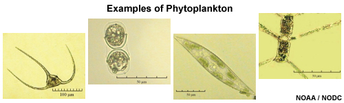
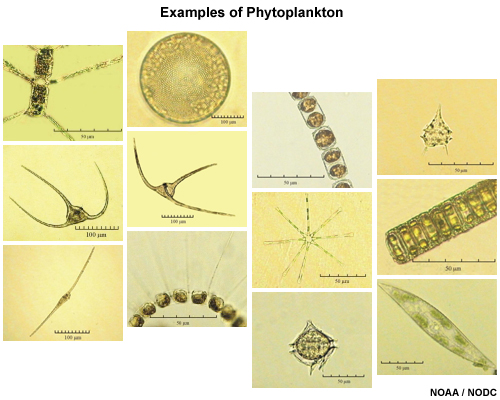
Like almost all other marine food webs, at the base of the Arctic marine food web are phytoplankton and zooplankton. Phytoplankton are microscopic plants (referred to as algae) that live in oceans and lakes (and swimming pools!). They serve as the primary food source for aquatic life and they consume carbon, an element which has a large influence on global climate.
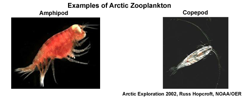
Zooplankton are microscopic animals that feed on phytoplankton. They in turn are food for larger organisms like fish and whales. It is essential to understand what is happening to phytoplankton and zooplankton because they are the foundation of the food web. They are being exposed to unprecedented conditions and it is not known how they will respond.
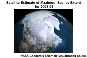
Sea ice is ice that forms on the surface of the ocean when ocean water freezes. Ice affects the amount of light that enters the ocean's surface and is available for phytoplankton to grow. Sea ice is also an important habitat for organisms from ice algae to seals and whales.
We can study polar phytoplankton and zooplankton by using computer models to predict phytoplankton growth and zooplankton "grazing". The knowledge gained from such studies will help scientists understand the fate of marine organisms as temperatures warm. Additionally it will help us understand how phytoplankton themselves affect the climate, now and in the future.
This module uses a computer model to simulate a simple Arctic ecosystem. The user can vary the model parameters to see for themselves what the most important variables are and how the ecosystem responds to differing environmental conditions.
Background
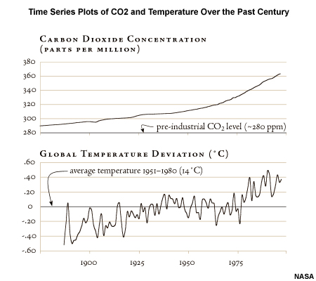
Over the past 150 years, the amount of carbon dioxide (CO2) in the atmosphere has dramatically increased due to human activities such as driving cars and burning coal and oil for energy. This increase in CO2 in the atmosphere is significant to humans and most all living things on Earth because CO2 acts to keep the Earth warm by absorbing outgoing thermal radiation and re-radiating it back to the surface. This is the so-called Greenhouse Effect. Higher amounts of CO2 in the atmosphere will lead to warmer temperatures in most places around the world. But scientists are not certain how exactly this change will affect the climate and organisms living on Earth.
Arctic Ecosystems
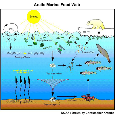
This diagram shows a simple representation of the Arctic food web: the complex arrangement of predator-prey relationships within an ecosystem. In the most elemental link, phytoplankton use energy from the sun to combine CO2 from the atmosphere with water to create glucose, a simple sugar. This process is called photosynthesis. Through this simple conversion of solar energy to food, they form the beginning of the entire food web. For this reason, we call the phytoplankton primary producers.
Moving up the food chain, zooplankton graze on and consume phytoplankton, and sometimes each other! Many animals consume zooplankton, including fish and birds. Of course, larger fish eat smaller fish, seals eat all fish, and polar bears eat seals.
Phytoplankton, zooplankton, and other animals that evade being consumed eventually die and fall to the seafloor. Some are consumed by scavengers, others by bacteria. In this way, most carbon-rich material that falls to the seafloor is recycled and kept within the ecosystem. The rest is buried with the sediments.
Open another view of the Arctic Ecosystem in a new window.
Open a summary graphic of photosynthesis in a new window.
The Carbon Cycle
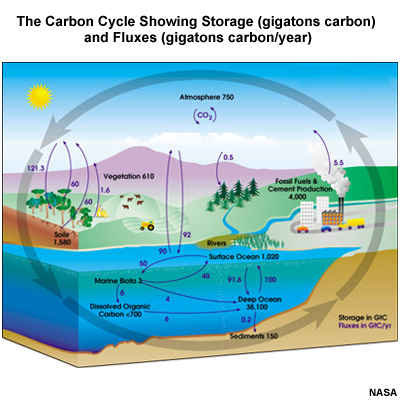
Understanding the ecosystem and food web is an important step in quantifying the carbon cycle. Carbon dioxide levels in the atmosphere are important because it’s a greenhouse gas. This means that when there is more of it, it acts to keep the earth warmer than it would otherwise be.
This graphic shows the major repositories and exchanges of carbon. By far, the largest repository of carbon is dissolved carbon dioxide in the deep ocean. Exchanges between the surface ocean/deep ocean and surface ocean/atmosphere are some of the largest in the carbon cycle. These exchanges are strongly affected by ocean ecosystems.
Phytoplankton
In the Arctic ecosystem, phytoplankton consume carbon when they photosynthesize. Much of this carbon comes from the atmosphere.
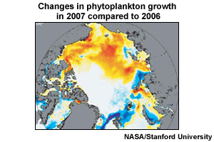
Warming climate and elevated levels of CO2 will affect the growth of phytoplankton in polar oceans in many ways. Phytoplankton, in turn, consume carbon and thus affect the amount of CO2 in the atmosphere, which affects the climate. This is called a feedback.
In addition to being the base of the food web, phytoplankton are important recorders of past climate. If we understand the factors that affect their growth, ancient plankton from deep sea cores can tell us what the Earth's climate was like in the past and how fast it changed. Thus, having a better understanding of phytoplankton growth at present can help us understand past and future changes.
The knowledge we gain from studying the growth of phytoplankton is important in understanding how future warmer temperatures may affect their growth. This, in turn, will help us understand how these microscopic plants in the ocean affect the climate around the world. The fate of phytoplankton will influence most other organisms that depend on these microscopic plants as a food source.
Sea Ice
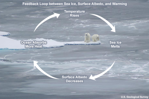
The polar regions are expected to be particularly sensitive to warmer temperatures. Higher levels of CO2 in the atmosphere lead to warmer temperatures in most parts of the world, including warmer temperatures in the world's oceans. Not only do surface waters heat up, but patterns of ocean circulation change, and sometimes warm water flows into a region that used to have cold water. These warmer temperatures melt more sea ice than usual in the summer and cause less sea ice to form in the winter.
Additionally, sea ice has a particularly strong feedback within the climate system. Sea ice reflects 50-90% of the sunlight that strikes it, absorbing little energy. Meanwhile, open ocean reflects less than 10% and absorbs the rest*. When there is less ice, the ocean absorbs significantly more solar energy and warms up more, causing more ice to melt.
The ice provides important habitat for polar bears and seals, as well as microscopic organisms like ice algae (algae that live within or attached to sea ice). Changes in sea ice will have a dramatic effect on life on earth, determining the fate of sensitive species such as polar bears, and influencing climate in places as far away as the equator.
A Warming World
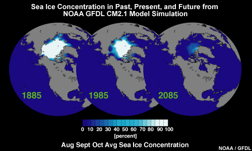
In the future there will very likely be less sea ice in the Arctic and warmer water temperatures. This is already affecting Arctic ecosystems in a number of ways and is expected to continue. However, no one is certain what the consequences of climate change will be.
- Larger carnivores will likely lose habitat
- Phytoplankton will have more light and warmer waters, thus will likely grow more. But different species might do better than others, and alter the food web from the base up.
- Increased CO2 in the atmosphere is likely to make the oceans more acidic. This may acutely impact animals with shells of easily dissolved calcium carbonate, including mollusks, corals, and many phytoplankton.
The Arctic Ecosystem
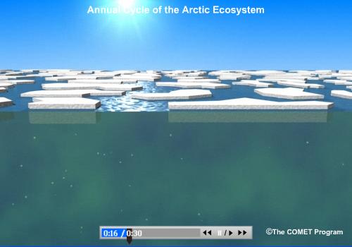
Click image to view animation.
This animation illustrates a simple nutrient-phytoplankton-zooplankton-detritus open-water ecosystem where phytoplankton grow based on light and nutrient availability (iron, nitrogen, phosphorus). Phytoplankton are grazed by zooplankton, with zooplankton dying off and becoming detritus. The detritus is eventually remineralized, turning back into nutrients, although the animation does not capture this microscopic scale. The animation shows a hypothetical polar ecosystem starting in the spring when sunlight first appears and begins to melt the sea ice, and following all the way through to late fall when daylight begins to fade and the ice re-forms. Notice how light in the water changes during different seasons and depending on sea ice cover, and now the water gets more or less “green” – indicating phytoplankton growth – in response to changes in light penetration.
How to Read the Model Results
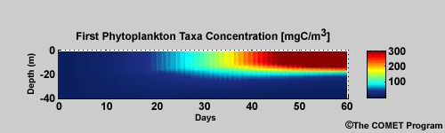
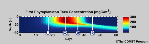
The model results are presented as a series of time-depth cross-sections, one for each model component. This plot shows one such cross section for phytoplankton abundance. The vertical axis is the depth. The horizontal axis shows the time. The abundance or concentration of the particular component is shown with color, in this case milligrams of carbon per cubic meter of seawater. Different color scales are available through the model interface.
Concentration versus Time and Depth
This plot shows a period of explosive population growth of the phytoplankton community, also known as a plankton bloom, in a simple model run with only phytoplankton and nitrogen (not shown).
1 of 2
When is plankton most abundant? (Choose the best answer.)
The correct answer is (c) Day 45.
The abundance of phytoplankton is measured as milligrams of carbon per cubic meter of seawater (mgC/m3). The highest concentrations are shown in dark red. The lowest concentrations are shown in dark blue. The highest concentrations occur near the end of the model run time. Thus (c) Day 50 is the best answer. On day 10, the color is dark blue, indicating a biomass concentration still near zero: the bloom had not yet started. At day 30, the color is a light blue, indicating the concentration is near 100 mgC/m3: the bloom had started, but had not yet reached its peak.
2 of 2
On day 45, at what depth is plankton most abundant? (Choose the best answer.)
The correct answer is (a) 10 m.
On day 45, at 10 m depth, the plot shows a deep red color, indicating a phytoplankton biomass concentration exceeding 300 mgC/m3. At 20 m, there is a sharp decrease in the biomass concentration to values approaching zero. Overall this plot shows a phytoplankton bloom with a rapid rise in phytoplankton biomass from near zero to over 300 mgC/m3 over a 20-day period starting at about day 20. The bloom is confined to the top 20 m of water, and most concentrated in the top 15 m.
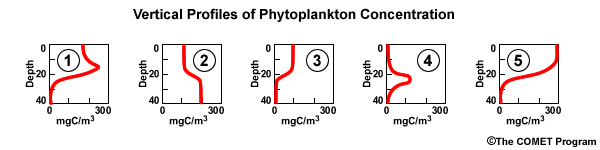
Results as a Series of Vertical Profiles
We can also view the time-depth vertical cross section as a chronological series of vertical profiles (i.e., a time series). This plot also shows phytoplankton biomass for a model run with nitrogen, phytoplankton, zooplankton, and detritus as components. The vertical lines on the plot mark the location of vertical profiles.
For each location (A,B,C,D) choose the correct vertical profile (Profile 1 - Profile 5)
1 of 1
(Select the appropriate vertical profile for each location on the map.)
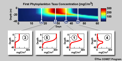
The correct answers are:
- Location A = Profile 3
- Location B = Profile 5
- Location C = Profile 1
- Location D = Profile 4
Model Components
In this section we run the model with different components turned on and off. We see how all the pieces fit together and how the model ecosystem works. We will use default values for the various model parameters.
Click "Launch Model" using the link below. Click "Launch Model" at the bottom of the menu at left. The model will appear in a different window (or tab, depending on how your browser is configured). Then work through this section turning on and off various components as required and examining the results.
Nitrogen and Phytoplankton
In the model menu, open Components (click on the "Components" heading in the left frame) to see the components selected. Nitrogen and Phytoplankton#1 are selected permanently. De-select all other default components and click "Run Model"
Phytoplankton grow in the surface where the light is, using up nutrients (in the model we track nitrogen). The phytoplankton growth causes nitrogen concentrations to decrease from 5 to 0 μM. Phytoplankton stop growing (at greater than 300 mg carbon/m3) because they have used up all the nitrogen. Phytoplankton die and turn back into nitrogen based on their mortality rate (you can see this if you set the "Run time", under the Model Settings tab, to 240 days). Light in the surface goes up and down throughout the day with the sun. The amount of sunlight also changes with the seasons. Light attenuates (diminishes) in the water column, so the deeper you go, the less light there is.
Nitrogen, Phytoplankton, Zooplankton
Now, add Zooplankton as a component and run the model (click on the "Components" heading if the arrow next to it is pointing down to expand the menu and check the box next to Zooplankton). Click "Run Model" again. How do the results differ?
Phytoplankton are eaten by zooplankton, decreasing the concentrations of phytoplankton back down toward zero, while zooplankton concentrations rise to greater than 300 mg carbon/m3. Zooplankton concentrations decrease based on their mortality rate. (In the absence of detritus, zooplankton turn directly back into nitrogen.)
When zooplankton eat the phytoplankton they graze with “sloppy feeding” and do not assimilate all of the phytoplankton into zooplankton. The remaining phytoplankton turn back into nutrients.
Nitrogen, Phytoplankton, Detritus
Add detritus as a component (and de-select zooplankton if they are still selected).
Instead of the oversimplified scenario of phytoplankton turning directly back into nitrogen when they die, phytoplankton turns into detritus (dead stuff). The detritus is then remineralized and turns back into nitrogen, adding one more step to the cycle. If the remineralization rate is set to 0, none of detritus returns to the environment as nutrients.
Run the model and compare the ecosystem with and without detritus as a component.
Nitrogen, Phytoplankton 1, Phytoplankton 2
Add Phytoplankton#2 as a component (and de-select any other components if they are still selected). Run the model and compare the ecosystem with one and two phytoplankton taxa.
If the two phytoplankton taxa have the same settings, each will grow equally and use up half of the nitrogen. If the phytoplankton have different settings, they will compete against each other for resources (nitrogen and light) and one will do better than the other. We will discuss the phytoplankton settings and their effect later, in the Sensitivity Experiments.
Nitrogen, Phytoplankton, Zooplankton, Detritus
Run the model with Nitrogen, Phytoplankton, Zooplankton, and Detritus as components. Compare the model results with those using fewer components.
With zooplankton and detritus switched on at the same time, the concepts are still the same, it is just adding complexity simultaneously. In this case, phytoplankton grow and use up nutrients. Phytoplankton are eaten by zooplankton. The biomass left over from “sloppy feeding” turns into detritus. Zooplankton die and turn into detritus. Detritus remineralizes and turns back into nitrogen, completing the cycle.
Nitrogen, Phytoplankton 1, Phytoplankton 2, Zooplankton, Detritus
Now turn on all components and run the model.
With all the components of our model enabled, our food web is complete. Of the scenarios we have examined, this one presents the most accurate representation of what happens in nature. Of course, ocean food webs in nature are much more complex than this simple example and include other organisms, including fish, seals, and polar bears.
In the next section we will begin varying other model parameters.
What the Model Shows
Sensitivity Experiments:
For each of these suggested experiments, before you run the model, make up a hypothesis of what you think will happen and why. Then run the model. What happened? Is this what you expected? It will be easiest to compare the model results if each time you click "Reset Values", then make your change and then hit "Run Model"
Model Settings
Depth - Depth of the modeled ocean.
This sets how deep in the water column the ocean the model will make its calculations. Most of the action will happen near the surface. You may want to increase or decrease the depth to better view the results.
Run Time - Length of model time the model will run.
This sets how long the model will run for in days. Some model setup will take longer to develop, and you might need to extend the model runtime to see what is happening. It is a tradeoff, however, because a longer "Run time" will mean you'll have to wait longer to get your results.
Timestep - Model timestep.
This sets the number of calculations the model makes for a given runtime. If it's too small, the model will take a lot longer to run. If it's too large, you will sacrifice accuracy.
Start Day - Day of the year for model start.
This sets the day of the year for the model to start on. There are different amounts of sunlight at different times of year.
| Calendar day | Day of year | Calendar day | Day of year | Calendar day | Day of year |
|---|---|---|---|---|---|
| January 1 | 1 | May 1 | 121 | September 1 | 244 |
| February 1 | 32 | June 1 | 152 | October 1 | 274 |
| March 1 | 60 | July 1 | 182 | November 1 | 305 |
| April 1 | 91 | August 1 | 213 | December 1 | 335 |
Latitude - North latitude in degrees.
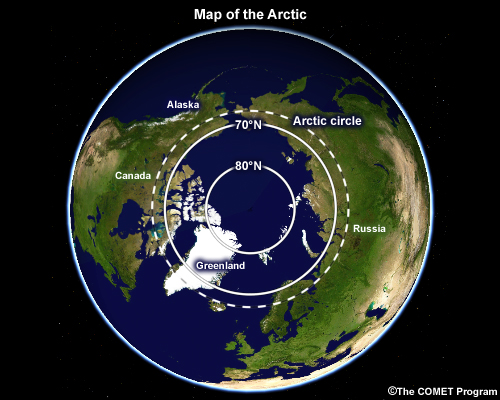
This sets the latitude for the model. We are running the model for the Arctic which is around 70° to 90°.
Ocean Settings
Ice Concentration - Sea ice concentration over the water.
Concentration of sea ice over the water column. A value of 0 is ice-free and a value of 1 is completely ice covered. Sea ice floats on the surface of the water and affects the amount of light that can reach the surface of the ocean.
Vary ice from 0 to 1. What happens? Why?
Ocean Temperature
Phytoplankton growth rates are dependent on temperature.
Vary temperature from -4° to 25°C. What happens to the timing of the bloom?
Initial Nitrogen - Initial nitrogen concentration in the water.
In this example, initially, the concentration of nitrogen is set to 5 μM everywhere in the ocean. This initial amount is the total available at any time in the model run and determines the total biomass that can accumulate.
Vary initial nitrogen from 0 to 20. What happens to the timing of the bloom? What happens to the magnitude of the bloom?
Remineralization Rate - Proportion of dead phytoplankton, zooplankton, and detritus that remineralizes to nitrogen per day.
The remineralization rate determines how fast detritus (dead stuff) remineralizes (gets transformed back into nutrients like nitrogen).
Vary remineralization rate from 0 to 0.5. What happens to nitrogen concentrations? Why? (you may have to increase the runtime to see what happens)
Phytoplankton Settings
K for Nitrogen - Determines how well the phytoplankton grows at low levels of nitrogen.
A lower K value means that growth is closer to maximum growth rates for a given nutrient level.
Vary the half-saturation coefficient from 0 to 2. What happens to the peak of the phytoplankton bloom? What happens to the magnitude of the bloom? Why?
(Click to see a detailed explanation. (Click to see a detailed explanation. Note: use your browser's back button to return to this location in the module.)
Ekmax - Reflects the amount of photosynthesis a plant can undergo at a certain light level.
Phytoplankton are light limited if there is not enough light available for them to grow at their maximum rate. Lower Ekmax values mean that phytoplankton approach their maximum levels of photosynthesis at lower light levels.
Vary Ekmax from 10 to 500. What happens to the depth of the bloom? What happens to the timing? Why?
(Click to see a detailed explanation. (Click to see a detailed explanation. Note: use your browser's back button to return to this location in the module.)
Growtho - Temperature-specific growth rate.
The temperature-specific growth rate determines the temperature-dependent maximum growth rate. When Growtho is low, it means that phytoplankton don’t grow well at a given water temperature. When it is high, it means they grow much better.
Vary from 0.4 to 1.0. What happens to the magnitude and timing of the bloom?
(Click to see a detailed explanation. (Click to see a detailed explanation. Note: use your browser's back button to return to this location in the module.)
Carbon to Nitrogen - Carbon to nitrogen ratio.
Phytoplankton are composed of carbon, nitrogen, and phosphorus in a ratio of approximately 106:16:1. As a result, when phytoplankton consume nitrogen, they are also consuming about 6 times as much carbon. But this ratio of carbon to nitrogen varies in phytoplankton and here you can experiment with it yourself.
Vary from 3 to 12. What happens to phytoplankton and nitrogen?
Mortality Rate - Phytoplankton mortality rate.
The morality rate is how quickly phytoplankton die. When this value is high they are dying quickly. When zooplankton is turned on, phytoplankton are lost only to grazing and not to mortality.
(Vary 0 to 0.5)
Zooplankton Settings
K for Phytoplankton - Concentration of phytoplankton at which grazing is half of the maximum grazing rate.
Lower values of K mean that growth is closer to maximum growth rates for a given concentration of phytoplankton.
Vary from 40 to 150. What happens to zooplankton concentrations? What happens to the timing and magnitude of the phytoplankton bloom?
(Click to see a detailed explanation. (Click to see a detailed explanation. Note: use your browser's back button to return to this location in the module.)
Feed Minimum - Feeding threshold of phytoplankton.
Feed Minimum is the feeding threshold for zooplankton grazing on phytoplankton, expressed as Mg carbon per cubic meter of seawater. Below this concentration of phytoplankton, grazing is zero.
Vary from 0 to 100. What happens to phytoplankton and zooplankton?
Grazing Maximum - Maximum grazing term (0.4 1/d)
This is the maximum grazing rate of zooplankton on phytoplankton, expressed as the proportion of phytoplankton consumed on a daily basis.
Vary from 0.1 to 0.6. What happens to the magnitude and timing of the phytoplankton bloom? What happens to zooplankton?
Assimilation - Zooplankton assimilation of phytoplankton.
This expresses how efficiently zooplankton convert grazed phytoplankton biomass into zooplankton biomass, expressed as a proportion per day. If zooplankton are sloppy feeders and a lot of the phytoplankton is wasted (becoming detritus) the assimilation value is low.
Vary from 0 to 1. What happens to phytoplankton and zooplankton?
Mortality Rate - Zooplankton mortality rate.
The mortality rate is how quickly zooplankton die (and become detritus).
Vary from 0 to 0.2. What happens to phytoplankton and zooplankton?
Start Day and Latitude
Turn on only nitrogen and phytoplankton. Vary the start day and latitude. How does light in the ocean change?
Nitrogen, Phytoplankton1, Phytoplankton2, Zooplankton
For each of these experiments set each variable to the same value for both phytoplankton taxa. Then for one variable at a time make one higher and one lower and see which taxa of phytoplankton does better. Why?
- K for Nitrogen
- Ekmax
- Growtho
- Carbon to Nitrogen
- Mortality Rate
Detailed Explanation of Terms
K for Nitrogen
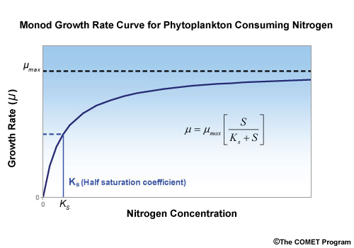
K is the half-saturation coefficient for Monod formulation uptake. In this case it is phytoplankton consuming the nutrient nitrogen. The half-saturation coefficient determines how well the phytoplankton can grow at low levels of nitrogen. Lower K values means that growth is closer to maximum growth rates for a given level of food.
This plot shows the the uptake rate (μ) of nitrogen by Phytoplankton as a function of the nitrogen concentration (horizontal axis). K is the nitrogen concentration where μ equals one-half of the maximum uptake rate (μmax). Logically, if K is smaller, the curve shifts to the left, meaning that the uptake rate (i.e., growth) is the same for a lower nitrogen concentration. Alternatively, this also means that the uptake rate is greater for the same concentration of nitrogen.
K for Phytoplankton
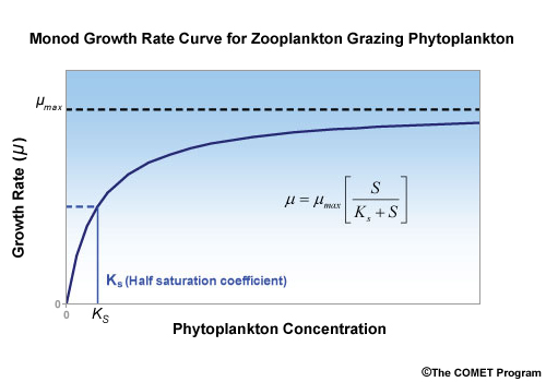
For zooplankton, the nutrient that they consume is phytoplankton. Thus, K (the half-saturation coefficient for Monod formulation uptake) operates the same for the phytoplankton consumed by zooplankton as it did for the nitrogen consumed by phytoplankton.
Growtho
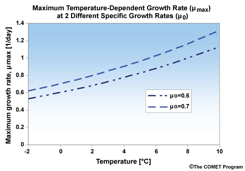
Growtho is the temperature-specific growth rate (μo), which determines the temperature-dependent maximum growth rate (μmax). When μo is low, it means that phytoplankton don’t grow well at a given water temperature. When it is high, it means they grow much better.
K and Growtho: 2 Phytoplankton Taxa
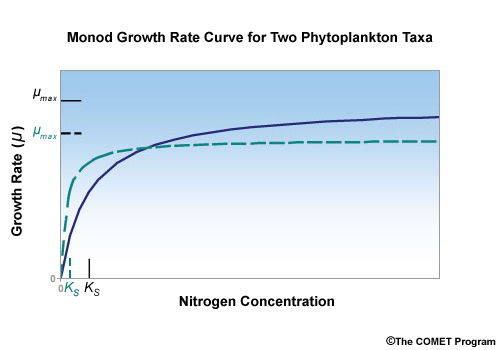
This graph shows the growth rate for two different hypothetical phytoplankton taxa. The taxa represented by the dashed line has a smaller μo (and hence a smaller μmax), as well as a smaller K for nitrogen. Notice that at low nutrient levels, the taxa represented by the dashed line displays a higher growth rate than the other solid-line taxa. However, at higher nutrient levels, the situation is reversed and the solid-line taxa grows more quickly than the dashed-line taxa.
Ekmax: Maximum photoadaptation parameter
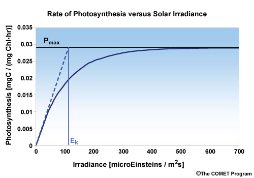
Ekmax is the maximum photoadaptation parameter. Ekmax reflects the amount of photosynthesis a plant can undergo at a certain light level. Phytoplankton are light limited if there is not enough light available for them to grow at their maximum rate. Lower Ekmax values mean that phytoplankton approach their maximum levels of photosynthesis at lower light levels.
Model Scenarios
Now that we have some understanding of the important elements of the Arctic ecosystem and how it operates, let's use the model to simulate some situations that may arise, both now and in the future.
Phytoplankton Competition
Read the following article online (opens in a new window):
Changing currents color the Bering Sea a new shade of blue. John Weir (1999) http://earthobservatory.nasa.gov/Features/Coccoliths/.
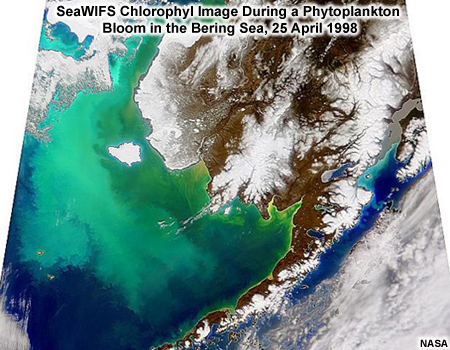
It's clear from this article that different environmental conditions can favor one species of phytoplankton over another, with potentially major repercussions.
How could you modify the phytoplankton input parameters so that one species is favored (and thus more abundant) when nutrient levels are high, and the other species is favored when nutrient levels are low? (Type your response in the box below.)
Answer
To favor one species when nutrient levels are low, increase its K for nitrogen.
To favor the other species when nutrient levels are high, increase its growth rate (Growth0).
Late versus Early Phytoplankton Blooms
Hunt et al., 2002 hypothesize that there are 2 states for the Bering Sea ecosystem.
(1) Late ice retreat (late March or later) leads to an early phytoplankton bloom in cold water (e.g., 1995, 1997, 1999).
(2) No ice, or early ice retreat (before mid-March), leads to a late phytoplankton bloom in warm water in May or June (e.g., 1996, 1998, 2000).
Zooplankton populations are not closely coupled to the spring bloom, but are very sensitive to water temperature. In years with an early bloom (Scenario 1), low temperatures limit the growth of zooplankton so that they are unable to take full advantage of the phytoplankton bloom. Alternatively, in years when the bloom is late (Scenario 2), it occurs in warm water and zooplankton populations should grow rapidly, feasting on abundant phytoplankton. This table summarizes these relationships:
| Ice Retreat | Late | Early |
| Phytoplankton Bloom | Early | Late |
| Water Temperature | Cold | Warm |
| Zooplankton Bloom | Small | Large |
How would you change the model settings to mimic early and late phytoplankton blooms?
What additional settings might you add?
(Type your response in the box below.)
Discussion
The ecosystem model we use here does an imperfect job of simulating the conditions described in this scenario. This results from two main factors: (1) the water in the model has a uniform temperature. It is not stratified (warmer at the surface and cooling with depth). (2) The growth rate for zooplankton (based on their grazing rate) is not temperature dependent. However, with those caveats, we can simulate this scenario as follows:
In order to simulate early versus late phytoplankton blooms, we can change the amount of light available for phytoplankton growth. This is most easily done by changing the sea ice cover. Remember that early ice retreat results in a late bloom. For an early bloom, we set the sea ice concentration to 50%. Then, for a late bloom, we set the sea ice concentration to 0%.
Because the zooplankton growth rate in the model, controlled by the grazing rate, is not temperature dependent, we need to set the grazing rate manually. Early ice retreat leads to warm water, so we use a higher grazing rate (0.4). Conversely, the late ice retreat results in cold water, with a lower grazing rate (0.2).
1 of 3
Which scenario favors an increase in the abundance of foraging fish that eat zooplankton? (Choose the best answer.)
The correct answer is (b) Scenario 2.
Because zooplankton are the primary prey for larval and juvenile fish, scenario (1) will limit the survival of larval/juvenile fish. Alternatively, in periods when the phytoplankton bloom occurs in warm water, zooplankton populations should grow rapidly, providing plentiful prey for larval and juvenile fish.
2 of 3
Which scenario favors an increase in the abundance of predatory fish that eat foraging fish? (Choose the best answer.)
The correct answer is (b) Scenario 2.
Fewer zooplankton in scenario (1) will limit the survival of larval/juvenile fish that grow into large predatory fish. When continued over longer periods, approaching a decade, this will lead to a decreased biomass of predatory fish (fewer and/or smaller fish). Alternatively, abundant zooplankton will support the survival of immature fish to maturity, which will lead to abundant predatory fish that control forage fish.
3 of 3
Which scenario favors an increase in the abundance of sea mammals and seabirds that eat foraging fish? (Choose the best answer.)
The correct answer is Scenario (1).
Fish-eating sea mammals such as northern fur seals and seabirds such as kittiwakes compete with predatory fish. When the number of predatory fish increases, the abundance of forage fish decreases, which leads to population declines in fish-eating sea mammals and seabirds. Thus, fewer zooplankton may actually help populations of fish-eating sea mammals and seabirds by limiting their competition for food from large predatory fish.
Reference:
Climate change and control of the southeastern Bering Sea pelagic ecosystem. Hunt, G.L. Jr., Stabenob, P., Walters, G., Sinclaird, E., Brodeure, R.D., Nappc, J.M., Bondf, N.A. Deep-Sea Research II 49 (2002) 5821–5853. http://www.ingentaconnect.com/content/els/09670645/2002/00000049/00000026/art00321
A Warming World
Li et al., 2009, found a trend in the Arctic Ocean of surface water warming and freshening. Deeper water remained unchanged. As the surface water warmed and freshened, nutrients decreased and the abundance of very small phytoplankton (picoplankton) increased, relative to larger phytoplankton (nanoplankton). The authors proposed that the warming and freshening of the surface waters increased ocean stratification and hence reduced mixing with nutrient-rich deep water. Reduced nutrients favor smaller phytoplankton because they have a higher surface-area-to-mass ratio so they are better able to take up nutrients at low concentrations than larger phytoplankton.
The authors see potential implications for this trend:
1. The picoplankton are so small that they essentially do not settle out of the water column. The least bit of turbulence will keep them in suspension. This reduces the amount of carbon that gets buried in sediments, with implications for the long-term carbon cycle.
2. The picoplankton are more difficult for zooplankton to harvest than larger phytoplankton. This alters the food web.
How would you change the model settings to mimic this change in the Arctic ecosystem? (Type your response in the box below.)
Answer
In an ecosystem with 2 phytoplankton taxa, zooplankton, and detritus:
Phytoplankton 1 (picoplankton): Decrease K for nitrogen because they are better able to take up nutrients at low concentrations.
Phytoplankton 2 (nanoplankton): Increase K for nitrogen because they are less able to take up nutrients at low concentrations.
Zooplankton find it difficult to graze on picoplankton, therefore we make the following changes:
- Increase K for phytoplankton: picoplankton are more difficult to graze.
- Increase feed minimum: picoplankton are more difficult to graze.
- Increase Assimilation: when eaten, less is wasted with picoplankton than with nanoplankton.
- Decrease grazing maximum: picoplankton are more difficult to graze.
What happens to zooplankton abundance? (Type your response in the box below.)
Answer
In a system described above, zooplankton abundance inevitably decreases. Zooplankton are prey for many other animals including whales, foraging fish, and some sea birds.
Reference: Smallest Algae Thrive As the Arctic Ocean Freshens. Li, W.K.W., McLaughlin, F.A., Lovejoy, C., and Carmack, E.C. (2009): Science, 326, (5952), 539. http://www.sciencemag.org/cgi/content/full/326/5952/539