Foundations of Global Navigation Satellite Systems (GNSS)

APPENDICES » APPENDIX 1: The mathematical solution of trilateration in two dimensions

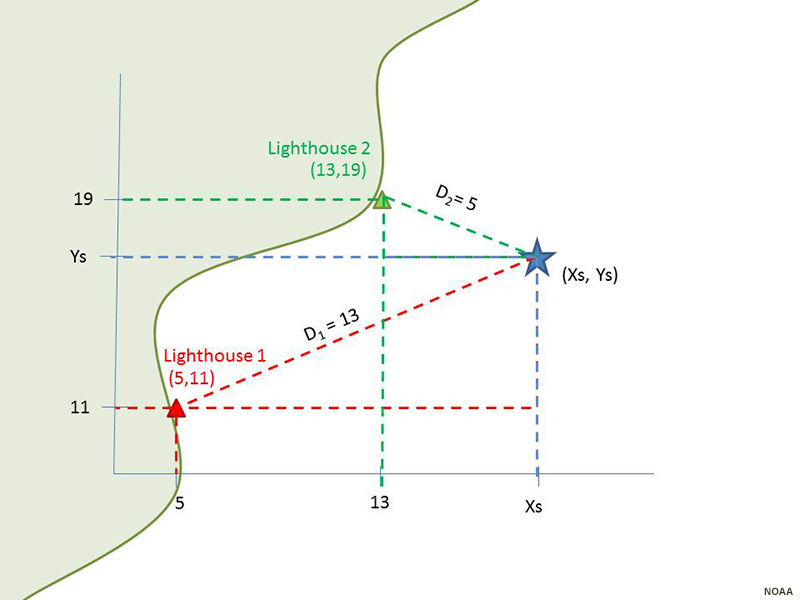
In our example of the boat off the coast receiving the audible signal from two lighthouses, we wanted to know the latitude and longitude corresponding to the position of the boat. In mathematical terms, the latitude and longitude can be expressed in the two-dimensional Cartesian Coordinates X and Y. These are the two variables we wish to solve for. Note that the positions of the lighthouses can be plotted in the same plane:

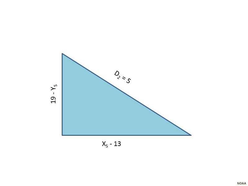
To solve for the unknown position of our boat, we use the Pythagorean Theorem to express the distances we computed from the signals into geometric relationships with respect to the light houses. The Pythagorean Theorem expresses the relationship between two sides of a right triangle and the hypotenuse:

Equation 1:

Equation 2:

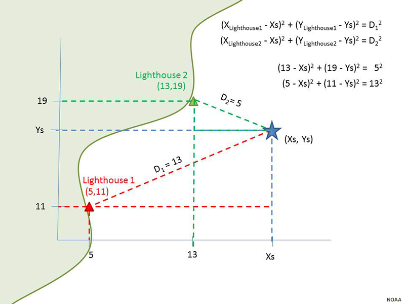
For Lighthouse 1, we would have the following geometric relationship:

Equation 3:

Similarly, for lighthouse 2:

Equation 4:

So we have our two equations and two unknowns.

Known:

Coordinates of Lighthouse 1 (5,11)

Coordinates of Lighthouse 2 (13,19)

Computed:

Computed distance between ship and Lighthouse 1 (based on the signal heard, 13 units)

Computed distance between ship and Lighthouse 2 (based on the signal heard, 5 units)

Unknowns:

Coordinates (X_S, Y_S) of ship

Solution:

Step 1: Define the two equations with two unknowns. We will eventually solve for the unknown position of ship (X_S, Y_S).

Equation 5:

Equation 6:

Step 2: We now have a system of equations: two equations with two unknowns. If the equations were linear (e.g., y = mx + b), this would be an easy solution. However, the equations are decidedly non-linear, so the solution is a lot more complex. One way of solving this is to linearize the non-linear equations using a Taylor Series Expansion of the square root function. Taylor Series are an infinite series, so we will only use the first (and most important) terms.

Apply a Taylor Series expansion to each distance equation (we need to linearize the nonlinear equation):

Equation 7:

Equation 8:

Equation 9:

Equation 10:

Note that the terms D₁(x_S, y_S) and D₂(x_S, y_S) refer to the observed distances (obtained by using the fog horn blasts from the two lighthouses). The computed distances refer to an initial estimate of the position based on where we think we are (called the “a priori” position estimate in GPS lingo).

Step 3: Take the partial derivatives of D₁ and D₂ with respect to x and then y:

Equation 11:

Equation 12:

Equation 13:

Equation 13b:

Substituting the Equations 5 and 6 into these partial derivatives (Equations 11-13) allows us to simplify these expressions:

Equation 14:

Equation 15:

Equation 16:

Equation 17:

Step 4: We can express the difference between the observed distance (the one we obtained using the sound blast and the speed of sound) and the computed distance in x and y (our unknowns):

Equation 18:

for i = 1, 2

Step 5: Since Appendix 1 Equations 7 and 9 are of the form

we can see that ΔD reduces easily to the form

Note that the differences (ΔD’s) are approximate from the Taylor Series’ expansions. The exact solution therefore specifies an error term, v:

Equation 19:

Substituting the simplified Equations 14-17 into Equation 19 yields the following expressions:

Equation 20:

Equation 21:

The reader can see that we have retained our two equations and two unknowns.

Step 6: This system of linearized equations can now be expressed in matrix form:

Equation 22:

This can also be written in the matrix form:

b = Ax + v

Where:

b is a matrix that contains the differences between the observed and computed distances

Ax is the cross product of the matrices that contain the unknown correction parameters for the positions.

The positional solution is contained in the matrix x, since these are the differences between the a priori estimates of the boat’s position and the unknown (true) position of the boat. Least squares approximation techniques are used to minimize the error matrix v, and the solution can be expressed as:

x = (A^TA)^-1 A^Tb

One can also solve the equations iteratively by hand, as is shown in the example below:

Back to our boat example: assuming we guessed that our initial starting coordinates were (15,15); we have the following “knowns:”

Variable	Value (km)
XLighthouse 1	5
YLighthouse 1	11
XLighthouse 2	13
YLighthouse 2	19
XBoat-estimated	15
YBoat-estimated	15
D1	13
D2	5

D₁ (observed) is 13 km. D₁ (computed) is obtained from the Pythagorean Theorem:

Equation 23:

Equation 24:

Taking the difference between the observed distances minus the computed distances, we arrive at:

Equation 25:

… and

Equation 26:

We can plug numbers into the system of equations (matrices described above) and come up with a set of two equations relating the differences between observed and computed distances (we omit the error term, as we will solve the system of equations iteratively):

Equation 27:

or

Equation 28:

and

Equation 29:

or

Equation 30:

We solve the first equation for Δx:

Equation 31:

and plug this into the second equation for Δy:

Equation 32:

or

Equation 33:

Plugging this value for Δy back into the first equation for Δx yields:

Equation 34:

We can now use these differences to get a better estimate of our position. Substituting these new values into the original system of equations will yield a second set of Δx and Δy, and thereby a third estimate of our position. Usually only a couple iterations are needed to obtain a convergent solution, X_S ≅ 17, Y_S ≅ 16.